Add an index column (Power Query)
- If you select the arrow and select From 0, you can start numbering the rows at 0.
- If you select the arrow and select Custom, you can enter a Starting Index and Increment to specify a different starting number and way to number each row.
How do I find the index of a column in Excel?
To apply the MATCH function to get the Excel table column index we need to follow these steps:
- Select cell H3 and click on it.
- Insert the formula: =MATCH(G3,Table1[#Headers],0)
- Press enter.
- Drag the formula down to the other cells in the column by clicking and dragging the little “+” icon at the bottom-right of the cell.
What is index formula excel?
The Excel INDEX function returns the value at a given location in a range or array. You can use INDEX to retrieve individual values, or entire rows and columns. The MATCH function is often used together with INDEX to provide row and column numbers. Get a value in a list or table based on location.
What is index in Excel sheet?
Summary. The Excel INDEX function returns the value at a given location in a range or array. You can use INDEX to retrieve individual values, or entire rows and columns. The MATCH function is often used together with INDEX to provide row and column numbers.
How do you calculate an index example?
To calculate the percent change between two non-base index numbers, subtract the second index from the first, divide the result by the first index and then multiply by 100. In the example, if the third-year index was 119.1, subtract 114.6 from 119.1 and divide by 114.6.
What is the index method?
The indexing method means the approach used to measure the amount of change, if any, in the index. Some of the most common indexing methods include ratcheting (annual reset), and point-to-point.
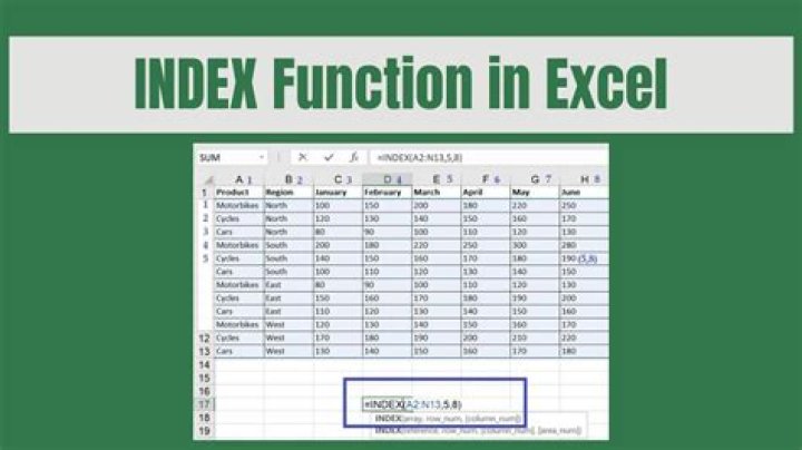
How do I find the index of a cell in Excel?
=MATCH() returns the position of a cell in a row or column….Follow these steps:
- Type “=INDEX(” and select the area of the table, then add a comma.
- Type the row number for Kevin, which is “4,” and add a comma.
- Type the column number for Height, which is “2,” and close the bracket.
- The result is “5.8.”


